DECISION TREE

 DECISION TREE

Have you ever wondered why ensemble algorithms give out the best results? Here is the answer to your question. The ensemble algorithms are the most powerful machine learning algorithms it combines multiple algorithms to solve the complex problems. Ensemble techniques are very useful to get the best results in competitions, Hackathons, and many more. Few ensemble algorithms are Random Forest, Gradient Boosting, and XGBoost. To understand these techniques you should know about the decision tree in depth.

In this article, I will be explaining,

• Introduction to Decision Tree
• Types of Decision Tree
• Attribute Selection Measures
• Example of Decision Tree
• Avoid overfitting in Decision Tree
• Implementation in Python

 

Introduction to Decision Tree

Decision Tree is a supervised machine learning algorithm that is used for solving both classification and Regression problems. It is like a tree-structured classifier that is upside down as shown in the figure.

Terminologies of Decision Tree

Root Node: Root Node is where the tree starts. It is the whole sample dataset, which gets divided into sub-nodes. It is also called the parent node.

Internal Node: The Internal nodes contain both the root node and the leaf nodes. It is also called the child node

Leaf Node: Leaf nodes are the final output of the decision tree, the decision tree cannot be split further after leaf nodes. It is also called terminal node.    

 

Types of Decision Tree

Depending on the dependent variable (i.e., output/ target variable) decision tree is classified into two types.

1. Regression Tree

A decision tree is used as a regression analysis when the dependent variable is continuous like house price prediction, an income of an employee, etc. 

 

2. Classification Tree

A decision tree is used for classification when the dependent variable is categorical like 1 or 0, spam or ham, etc.

Therefore, the Decision Tree is called the Classification and Regression Tree (CART).

Attribute Selection Measures

To choose the right root node among the given attributes and split the data to its complete depth (i.e.; till homogenous nodes are left) we generally use Attribute Selection Measures for splitting the nodes. Let’s start with different splitting methods in the decision tree.

 

1. Entropy

Entropy is to measure the impurity of the given data. It is used for calculating the purity of the node in the decision tree if the data is having categorical dependent variables. Lower the entropy value, the higher is the purity. It is denoted by H(S). The formula for entropy is

Entropy H(S) = -P ₍₊₎ log₂ (P ₍₊₎) - P _(-) log₂ (P _(-))

Where,

P ₍₊₎ = Total positive class

P _(-) = Total negative class

The Entropy value ranges from 0 to 1 as shown in the figure below.

2. Information Gain

Information Gain measures the change in entropy after the data is spilt based on an attribute (independent variables) if the data is having categorical dependent variables. Constructing a DT (decision tree) is for finding attribute that returns the highest information gain. It is denoted as IG(S, A). The formula for information gain is

IG(S, A) = H(S) – H(S, A)

Where,

H(S) = Entropy of the entire data

H(S, A) = Entropy for the particular attribute A

3. Gini Impurity

Gini Impurity is a method for splitting the nodes while creating a decision tree if the data is having categorical dependent variables. If the value of Gini Impurity is low then we consider higher the homogeneity of the node. For a pure node, Gini Impurity is zero. The formula is given as 

Gini Impurity is recommended for information gain, it is computationally efficient compared to entropy because it does not contain logarithms. The value ranges from 0 to 0.5 as shown in the figure below.

4. Chi-Square

Chi-Square is one of the methods for splitting the nodes in the decision tree if the data is having categorical dependent variables. This method is used to find out the statistically significant difference between the parent node and the child node. If the value of chi-square is higher, then the statistically significant difference between the parent node and child node is high. The formula for chi-square is

5. Reduction in Variance

Reduction in Variance is a method for splitting the nodes in the decision tree if the data is having continuous dependent variables. This method uses variance as a measure for splitting the data because it calculates the homogeneity of a node. The split is based on low variance. The formula for calculating variance is

Example

Steps for Decision Tree

1. Calculate the entropy of the class.

Entropy (PlayTennis) = Entropy (5, 9)

                                       = Entropy (0.36, 0.64)

                                       = - (0.36log₂ 0.36) - (0.64 log₂ 0.64)

                                       = 0.94

 

2. The entire data is split based on different independent variables. The entropy for each variable is calculated. The resulting entropy for independent variables is subtracted from the entropy of the class. The resulting value is the information gain (IG).

IG (PlayTennis, Outlook) = Entropy (PlayTennis) – Entropy (PlayTennis, Outlook)

                                            = 0.94 – 0.693 = 0.247

Similarly, Calculate for other attributes.

3. Now we have to choose the attribute with the highest information gain as the root node, from the above table, we can see that ‘outlook’ has the highest information gain, divide the dataset by its sub-nodes.

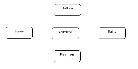
4. Repeat the same process for each sub node. The algorithm runs recursively on all sub-nodes until the entire data is classified.

The decision rules generated are:

Avoid overfitting in Decision Tree

Overfitting is one of the disadvantages of a decision tree. When a decision tree model is built on the entire data to its max depth it leads to overfitting the data (i.e., the training data accuracy is high but test data accuracy is low) which is also called low bias and high variance condition. To overcome the overfitting problem following methods are used.

1. Control tree Size
2. Pruning

1.  Control Leaf Size

Parameters play an important role while constructing a decision tree. Some of the regularization parameters are:

max_depth: This parameter is used to set the maximum depth of the tree.

min_samples_split: This parameter is used to set the minimum no of samples required to split the node.

min_samples_leaf: This parameter is used to set the minimum no of samples required at the leaf node.

max_features: This parameter is used to set the maximum no of features to consider for the best split.

2.  Pruning

Pruning is a process of reducing the size of the decision tree by eliminating the unnecessary nodes to get the optimal decision tree. There are two types of pruning.

i) Pre-pruning

Pre-pruning is a technique that prevents the insignificant nodes from generating by putting some condition when should it terminate before it classifies the data. It is also called forward pruning. 

 

ii) Post-pruning

The Post-pruning technique is applied to the generated decision tree and then the insignificant nodes are removed. A cross-validation metric is used to check the effect of pruning. It is also called backward pruning.

 

Note: In Decision Tree, no feature scaling is required, it is not sensitive to outliers and it can automatically handle the missing values.

 

Implementation in Python

Output:

To Download Code - Click Here